Contents
4 Geometry
4.1 BSplines
4.1.1 Terminology
4.1.2 Formulae
4.1.3 Class definition
4.1 BSplines
4.1.1 Terminology
Parametric and Sampled Curves
Parametric and sampled curves represent ordered sets of points in
2-D or 3-D space.
In the case of a parametric curve, it is possible to navigate along
all its points with a path parameter defined in a continuous interval.
We use C(t) to denote a point in such a curve.
We call path parameter domain the values which can be assumed by
the parameter t.
In the case of a sampled curve only some points are represented and
they are considered as linked with straight lines.
We use c[j] to denote a vertex in such curve, j being the index
in a vector of sampled points.
Parametric and sampled curves may be open or closed.
One type of parametric curve is called piecewise polynomial curve.
In this case each segment of the overall curve is given by two functions (or
three, in 3D) which are polynomials of degree d of the path parameter t.
Ex: polynomials for a 2D cubic piecewise polynomial parametric curve:
|
x(t) = ax t3 + bx t2 + cx t + dx |
| | y(t) = ay t3 + by t2 + cy t + dy |
|
|
A list of real values called knots define the space for the path
parameter t.
The coefficients a, b, c, d are computed from given information
(ex: control points) using a specific algorithm (or model).
Splines
Splines are parametric piecewise polynomial curves defined with a model
(the recipe) and control parameters (the ingredients).
They can be implemented with different methods to construct different types
of curves.
Examples: interpolating spline curves, B-spline curves, Beta-spline curves,
NURBS, etc.
B-Spline curves
We are actually interested in B-spline curves (see Figure 4.1), which
are splines implemented as a linear combination of basis functions
(see Figure 4.2).
We adopt the following terminology and notation:
- degree: degree of the polynomials (= order -1);
- type of curve: determine the usage of control points and knots at ends.
In closed curves, knots are used circularly.
There are several options for open curves, which we consider different types
of curves (ex. with loose ends or with repeated end points);
- knots: ordered list of values that define the path parameter values for
navigation along the curve.
The values of the knots may be initialized in different ways: uniformly or
non-uniformly distributed; generated automatically or explicitly informed by
the programmer.
- interval: piece of a curve determined by two path positions t1, t2.
- control points (P): geometry information used to instantiate a given
B-spline model as a curve in space.
The number of control points is dependent on the model, that is, the degree,
number of knots, and the curve type.
- basis functions (B): weight of control points for the computation of
curve points along the path. Basis functions are completely defined by
the knots and the degree of the curve. We refer to these as B(i).
- curve points (C): points in the parametric curve at hand.
In this implementation, curve points are never stored in the class, but
generated upon request.
In continuous curves, we refer to these as C(t).
In sampled curves, we refer to curve points as C(j), where j is the index
corresponding to a point with fixed t.
- derivatives (d): all derivatives are computed for the path parameter
t. We refer to these as dC(t, order), dB(i,t,order), etc.
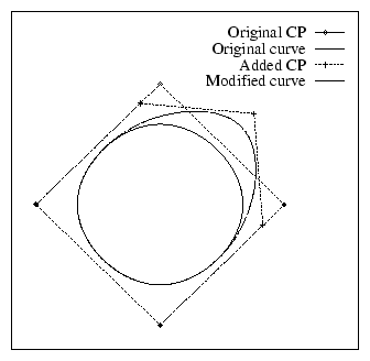
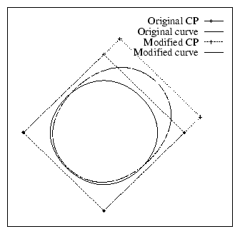
Figure 4.1: Examples of closed cubic B-Spline curves (degree=3).
Left: Curve with four control points and uniformly spaced knots.
Manipulation of one control point affects the whole curve.
Right: A control point is added (knots become unevenly spaced).
Manipulation of one control point affects only a curve interval.
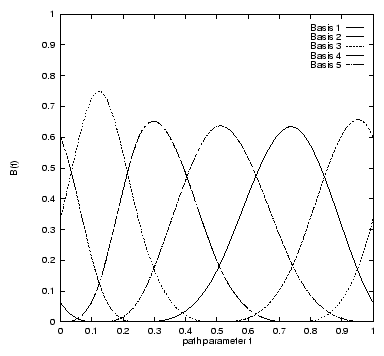
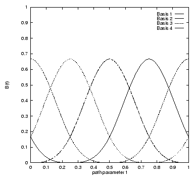
Figure 4.2: Basis functions for the curves in Figure 4.1.
Left: Uniformly spaced knots. Right: Unevenly spaced knots.
Introductory sources of information about B-splines are [1] and
[2], which we used as we used as an intermediate step.
Later we adopted [3] and [4].
The code follows the algorithm and notation as indicated in the comments.
Below we shortly present the most important formulae used in its implementation.
Keep in mind the following notation:
- d = degree
- o = order (d+1)
- ll = lth knot in the sequence
- t = path parameter
- Pi = ith control point
- Xi, Yi = x and y coordinates of control point Pi
- C(t) = curve point at t, (x, y) coordinates
- C(n)(t) = nth derivative of curve at path path parameter t, (x, y) coordinates
- Pi(n)(t) = contribution of ith control point for the computation of the nth derivative at path parameter t
- Bi, o(t) = value of ith basis function of order o at path parameter t
- Bi, o(n)(t) = nth derivative of ith basis function of order o at path parameter t
A curve point C(t), t ╬ [ll,ll+1), is evaluated as follows:
|
x(t) = |
l
Õ
i=l-d
|
Xi Bi, d+1(t) |
| | y(t) = |
l
Õ
i=l-d
|
Yi Bi, d+1(t) |
| (4.1) |
|
The value of a ith basis function of order o at position t - Bi, o(t), t ╬ [li,li+1) - is computed with the recursive method proposed by de Boor (see equation 1.24 in [3]):
|
|
|
|
|
t - li
li+o-1 - li
|
Bi, o-1(t) + |
li+o - t
li+o - li+1
|
,Bi+1, o-1(t) |
| (4.2) | |
|
|
|
The nth derivative of the curve at the path parameter t - t ╬ [ll,ll+1), is also computed with recursion
(see equations 1.39 and 1.40 in [3]):
|
C(n)(t) = |
n
š
i=1
|
(d + 1 - l) |
i
Õ
i=l-d+n
|
Pi(n) Bi, d+1-n(t) |
| (4.3) |
with
|
Pi(n) = |
ņ
’
’
Ē
’
’
Ņ
|
| |
|
|
Pi(n-1) - Pi-1(n-1)
ll+d+1-n - ll
|
|
| |
|
|
| (4.4) |
The value of the nth derivative of the ith basis function of order
o the path parameter t, t ╬ [li,li+1), is derived
from equation 1.25 in [3] and computed as follows:
|
|
|
|
(o-1) |
ņ
Ē
Ņ
|
|
Bi, o-1(n-1) (t)
li+o-1 - li
|
- |
Bi+1, o-1(n-1) (t)
li+o - li+1
|
³
²
■
|
|
| (4.5) | |
|
|
|
4.1.3 Class definition
The class design for the implementation is given in Figure 4.3.
Figure 4.3: BSpline curve classes
HxBSplineBasis
Class to represent the B-Spline basis functions, which correspond to the
``model.''
Internal Representation:
- degree: integer, │ 1.
- type of curve: closed, open (the ends are loose) or openRepeatEndPoints
(the end points are repeated, and the curve passes through them).
- range of path parameter: real, interval t ╬ [minT,maxT).
- knots: vector of increasing real numbers. The knots that define the
curve intervals are in the range [minT,maxT]. Extra knots are added to cope
with end point conditions for closed or open curves.
HxBSplineCurve
A HxBSplineCurve results from the association of a HxBSplineBasis with a vector of
control points used to instantiate it in 2-D.
Internal Representation:
- HxBSplineBasis: determines the curve model.
- vector of control points: instantiate curve in 2-D.
This curve is called continuous because its manipulation is valid for
any value of t ╬ [minT, maxT).
HxSampledBSplineCurve
A HxSampledBSplineCurve consists of a HxBSplineCurve and a vector of t values indicating
the path positions where the continuous curve is sampled.
This is meant to facilitate the manipulation of sampled curves.
Potentially, the implementation of a sampled curve allows for the
pre-computation of values to increase performance (e.g. curve points and basis).
The current implementation does not take advantage of this.
Internal Representation:
- HxBSplineCurve: the continuous curve.
- vector with sampled path parameter positions.
Bibliography
- [1]
-
T. PAVLIDIS.
Algorithms for Graphics and Image Processing, chapter
B-splines.
Springer-Verlag, 1982.
- [2]
-
J.D. FOLEY, A. VAN DAM, S.K. FEINER, and J.F. HUGHES.
Computer Graphics - Principles and Practice, chapter
Representing Curves and Surfaces, pages 471-532.
Addison-Wesley, 1990.
- [3]
-
P. DIERCKX.
Curve and Surface Fitting with Splines, chapter Univariate
Splines.
Oxford, 1993.
- [4]
-
L. PIEGL and W. TILLER.
The NURBS book, chapter Curve and Surface fitting, pages
361-454.
Springer, 1997.
File translated from
TEX
by
TTH,
version 2.89.
On 04 Feb 2003, 13:16.